Google Sheets: Best practices to prepare your data for your dashboard

Before you can analyze your data, make sure it has an analyzable structure and stays up to date. The cleanest approach is to organize data in a database-style layout and configure automatic updates from the source. These two steps let you spend less time fixing data and more time acting on it.

Database layout

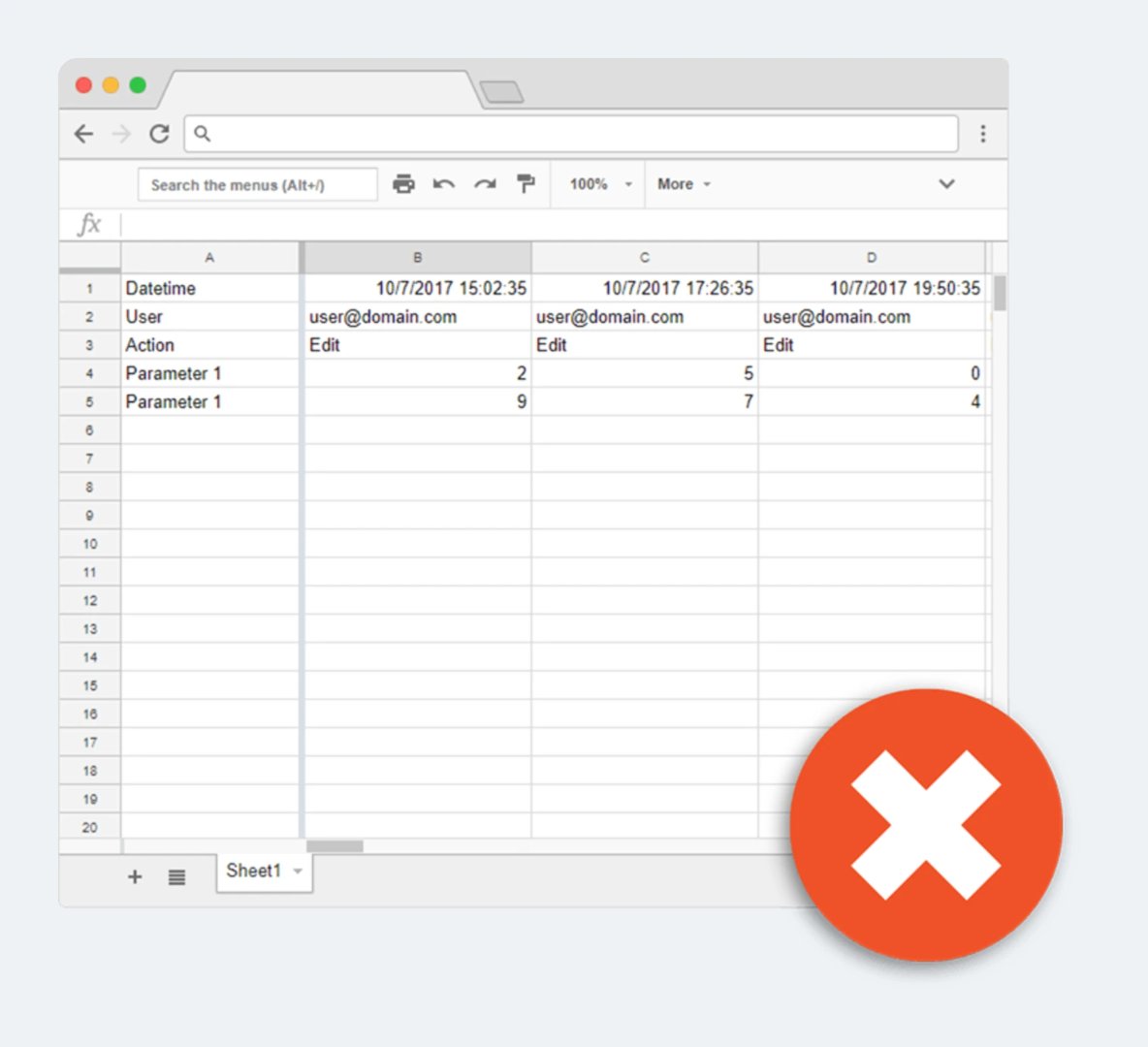
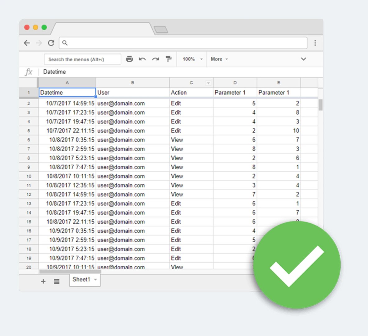
With Google Sheets, as with any spreadsheet software, you can choose the starting cell for your table. You could start a dataset on the fifth row and third column, but that creates friction later. Start in the first row and first column, with labels in row one and data listed vertically below. That structure is what most formulas and connectors expect.

Data format

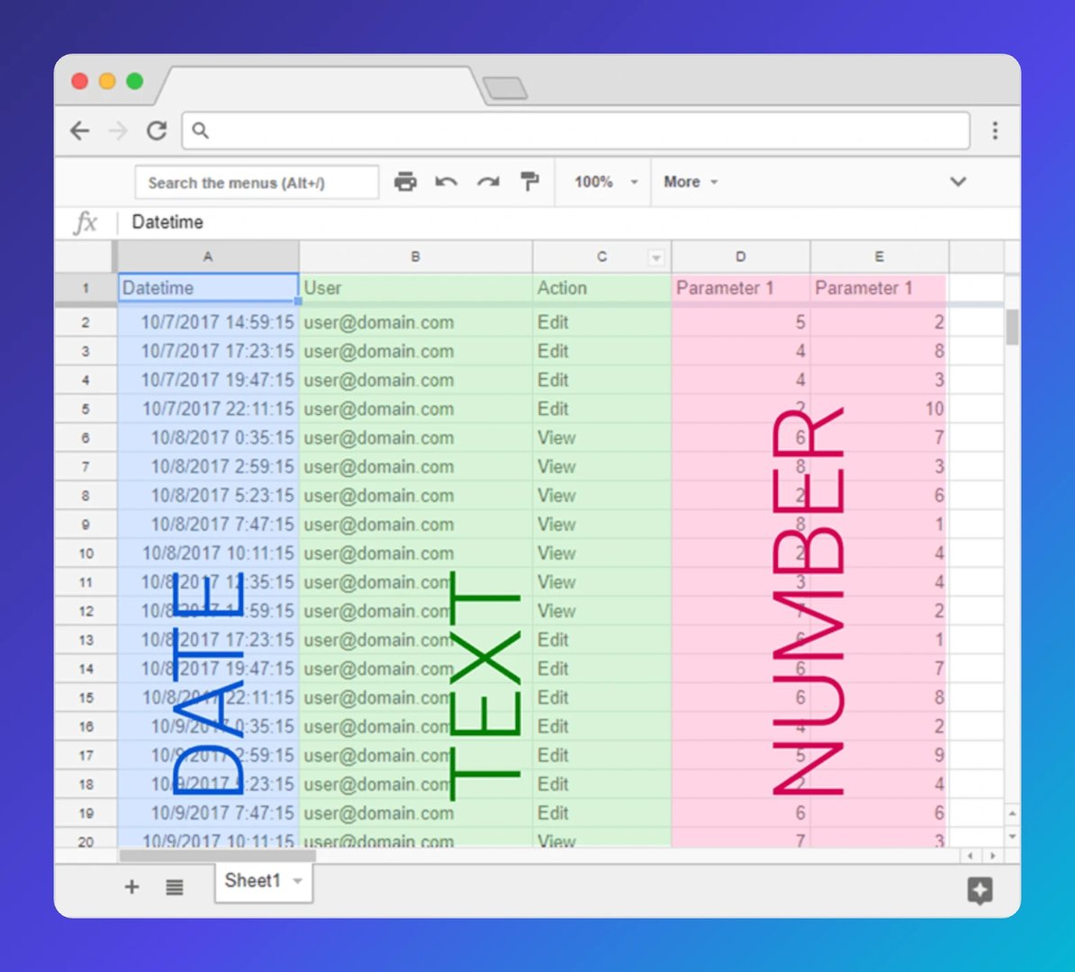
Each column should use a single data type. Set column A to dates, column B to currency, and so on. Set formats explicitly from the menu rather than relying on automatic detection. When Sheets guesses wrong, your formulas inherit the error and the numbers on your dashboard stop being trustworthy.

Automating the data transfer

The data you bring to a dashboard rarely lives in a single sheet. Many teams maintain dozens or even hundreds of spreadsheets that need consolidation. Copy and paste invites errors, wastes time, and means someone has to pull the number before you can trust it.

Two good options connect your data with Google Sheets and cut that risk. The first is the function ImportRange, and the second is a Google Sheets add-on called Sheetgo. ImportRange works well for small volumes of data and ad hoc analysis between spreadsheets. If connecting spreadsheets becomes routine and you depend on those links for ongoing reports and decisions, use a tool designed for data transfer like Sheetgo.

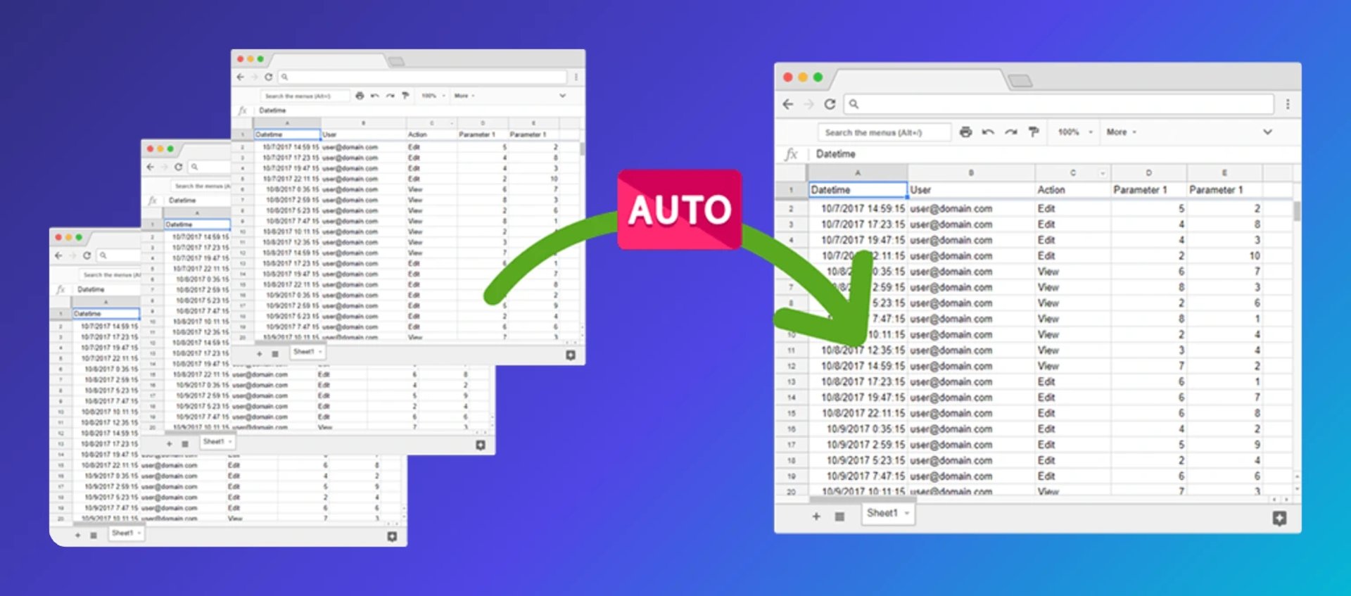
Automating the transfer means the number on your dashboard reflects reality without anyone having to remember to update it.

Infinite and automatic formulas

Google Sheets lets you plan for future data with a single formula so you don't copy the same calculation thousands of times. Use =ARRAYFORMULA() to replicate a formula across an entire range automatically.

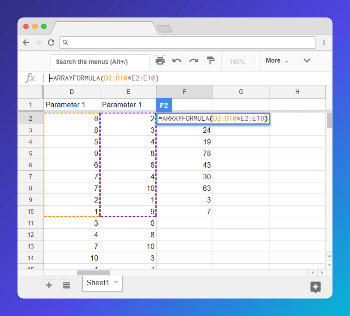
Two things to watch:

• Open-ended ranges and blank rows: When this formula targets an open-ended range, it applies your calculation down to the last row, including blank rows. That can trigger errors. Wrap the logic in an IF statement that checks whether the row has data; if not, return a blank.
• Range symmetry: If the formula reads from one area and writes to an overlapping area, Sheets may attempt to add infinite rows and crash.

Creating pre-analysis

If you want to track how many sales were made last week and need that number refreshed weekly, two techniques keep your data dynamic without manual intervention.

Infinite ranges

If the data you're analyzing has 1,000 rows today, you might write a formula over A1:A1000. As new rows arrive, you'd need to adjust the range manually. Remove the ending row number, like A1:A, and Sheets treats that as an open-ended range. The formula includes new rows automatically, so your dashboard stays current without anyone touching it.

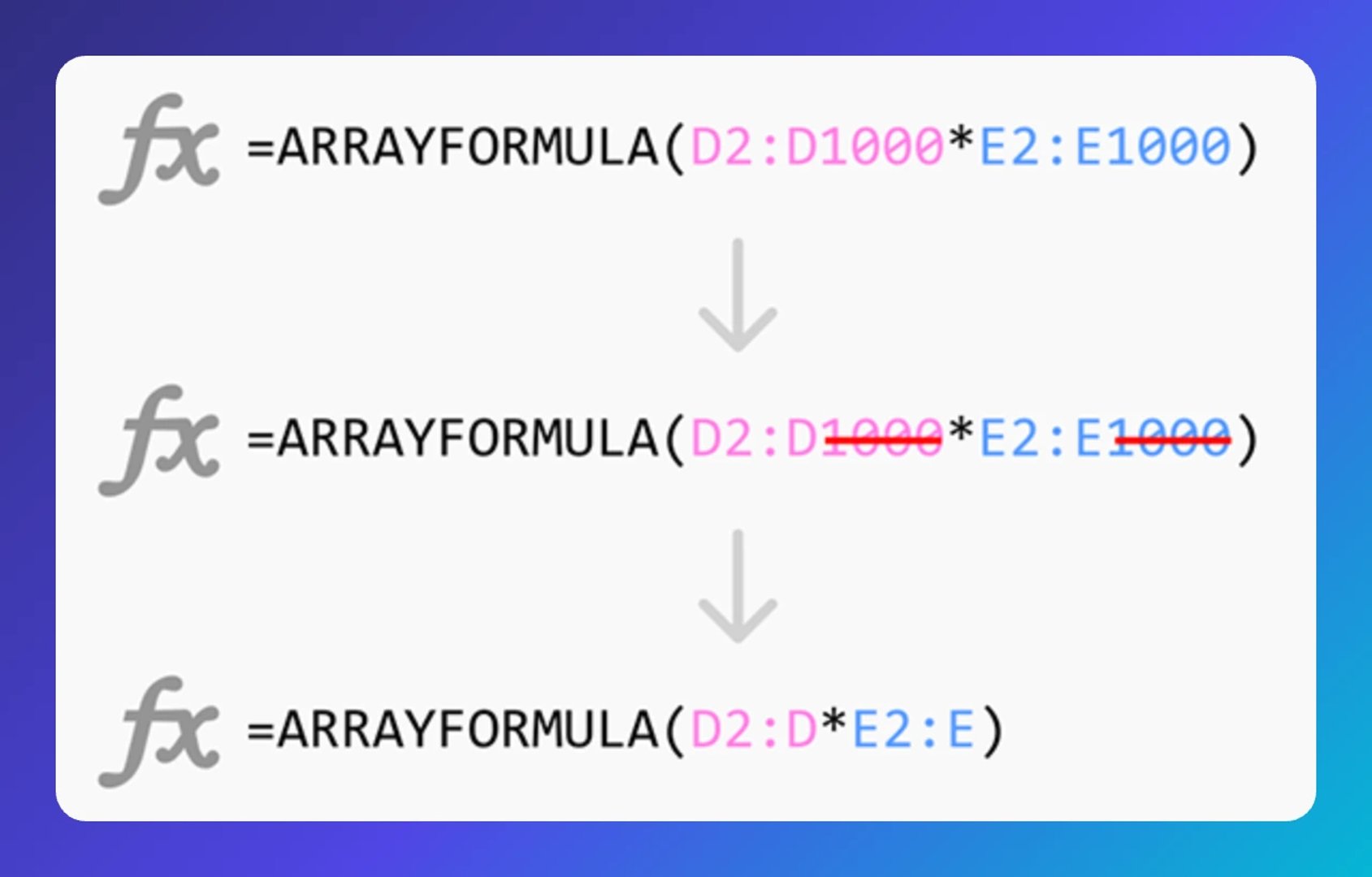
Rolling periods of time

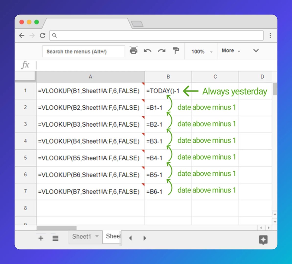
Say you need a 7-day sales view. List the dates in the first column and the daily counts in the second. To keep the window rolling, insert a dynamic base date and make the other dates relative. In cell A7 enter =TODAY()-1 (yesterday). In A6, reference A7 minus 1 (=A7-1), and continue until you show the last 7 days. Each day, the range shifts automatically so your dashboard always reflects the latest week without anyone having to check or update it.

Get your data into a dashboard

These practices give you a solid base: clean structure, consistent formats, automated transfers, and formulas that keep up with new data. The result is a sheet you can trust, which means numbers on your dashboard you can act on.

When you're ready to share results, Klipfolio Klips connects directly to Google Sheets and turns that clean data into dashboards your whole team can see, without anyone having to paste numbers into a report or explain the context from scratch. Get started for free.