5 Excel Tips and Tricks Every Marketer Needs To Know

Due to its pivotal role in handling data, Excel tips and tricks are everywhere.

But does that make Excel easy?

No way.

The program boasts a substantial amount of complex functions, formulas, and uses - like creating video games from scratch or crafting intricate art pieces.

But if you need to make data-driven marketing decisions, and you’ve got questions like:

• How do I organize a lot of data in Excel?
• What are the best Excel formulas?
• How do I extract data from multiple webpages/worksheets?

Using Excel can feel like a daunting task.

That’s why we’re going to explore the essential Excel tips and tricks every marketer needs to know inorder to make smart, incisive, and profitable data-driven choices.

Excel Tip 1: How to Use Pivot Tables To Draw Powerful Insights

The 2nd quarter has arrived, and you’ve been summoned to a quarterly meeting. You’ve been asked to present a detailed Excel report showing how the company is measuring up to its KPIs.

The problem: The Excel sheets holding the relevant data are a whirlwind of conversion rates, traffic stats, sales, and other metrics. How do you filter through this data to summarize progress and draw useful insights?

The answer: Create Pivot Tables.

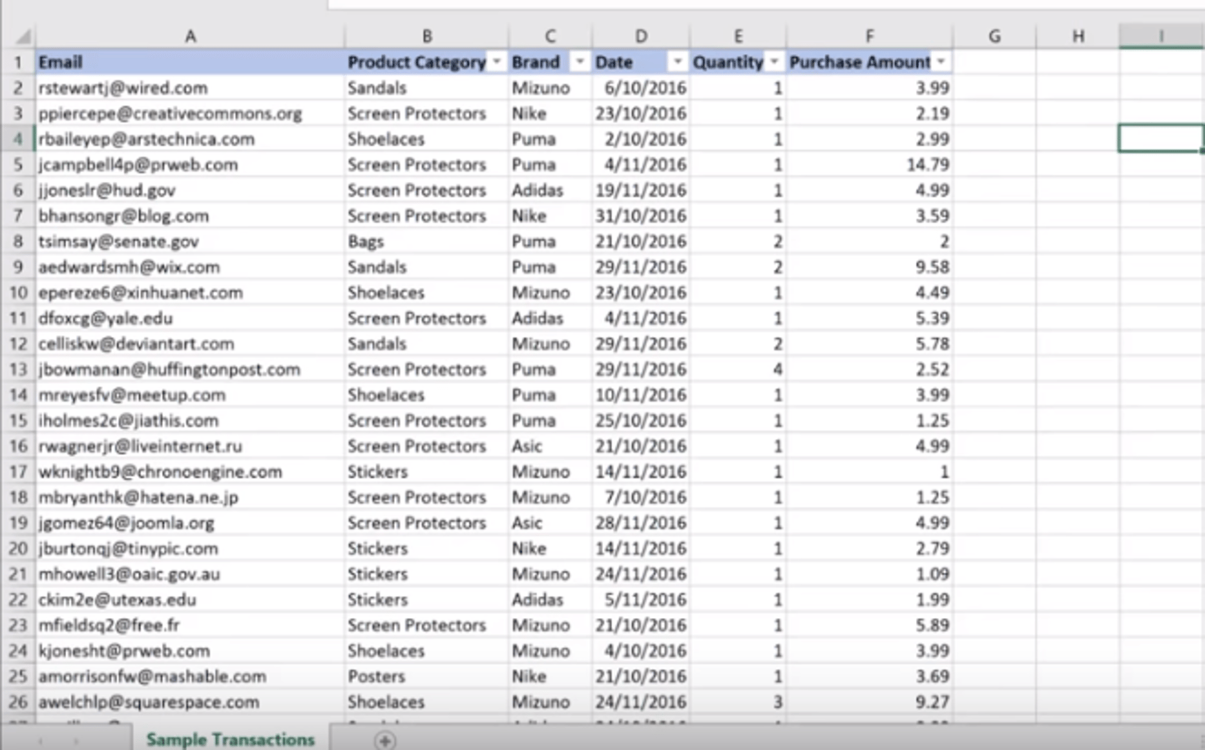
Pivot tables restructure data in a way that exposes positive or negative trends buried in large amounts of data, and data outliers. Take the sales and customer data in the spreadsheet below as an example:

Image Source

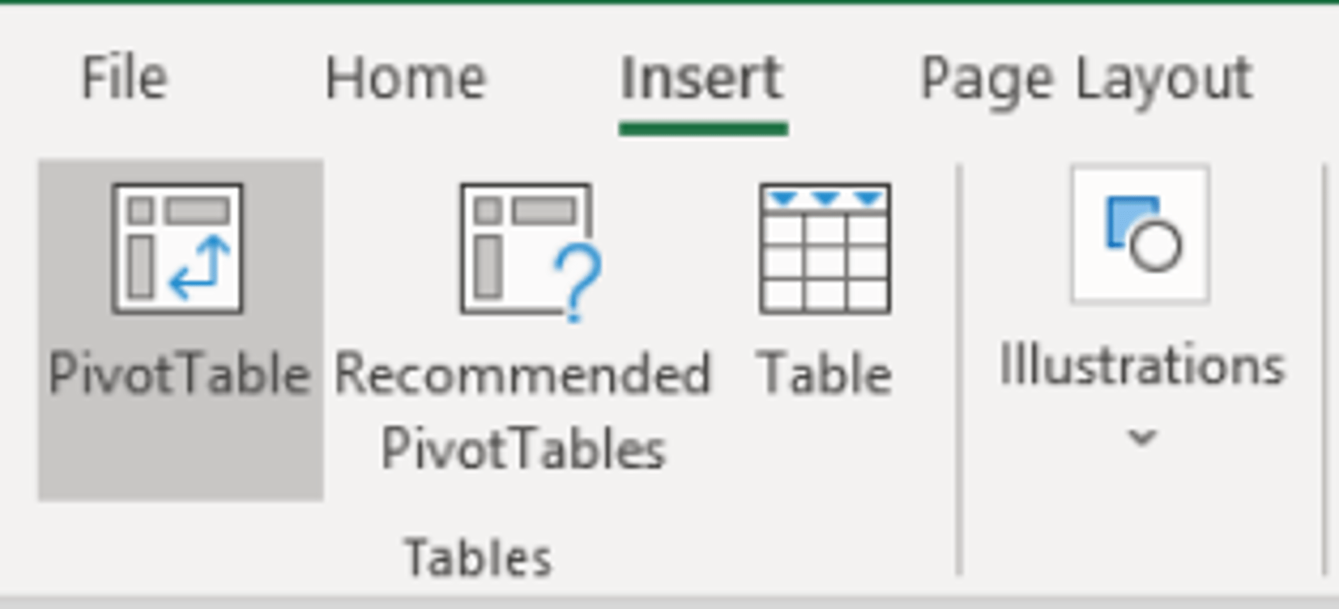
To compare the best/worst selling products, start by highlighting the data and select Insert, then choose Pivot Table.

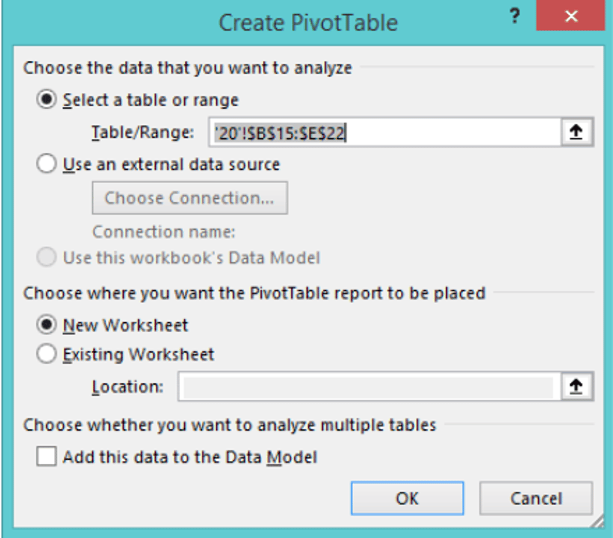
A dialogue box will prompt you to choose which data to analyze and where to place your pivot table.

You can then organize the data using four options:

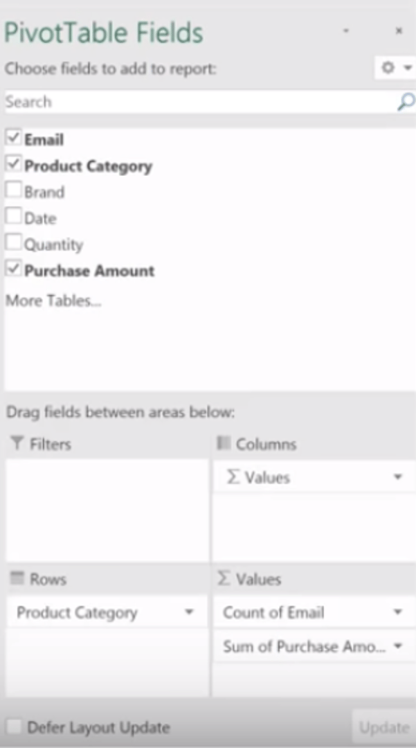
1. Row labels: Applies a filter to rows that have to be shown in the pivot table.
2. Column labels: Arranges headers in the pivot table you’re creating.
3. Value: Lets you customize the data selected by the row and column labels. The default option will be a sum, but you can choose between count, average, maximum, minimum, and a few other options.
4. Report filter: Applies a filter to an entire table. It allows you to alter the data that is summarized in the pivot table.

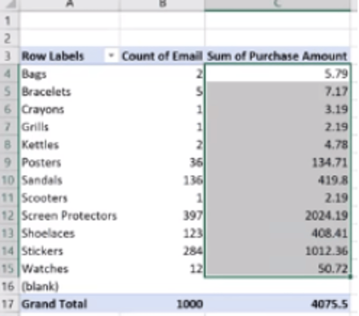
The completed table will look something like this:

Mini Excel Tip: By right-clicking on the respective field you have placed in the value field, you can tell Excel how to summarize each item in your row.

Excel Tip 2: How to Use VLOOKUP To Scrutinize Multiple Data Sources

Classed as a Lookup/Reference Function, VLOOKUP looks for a specified value in a column, and when it finds the specified match, it returns a value in the same row. This allows you to take data from a second spreadsheet and integrate it with the data in your first spreadsheet for deeper inspection.

You’ll need a unique identifier - unique information shared by both data sources, like an email address or name - before you can execute the function. The syntax for the VLOOKUP function is:

VLOOKUP(lookup_value , table_array , col_index_num , range_lookup)

To execute the function:

1. Choose a column of cells you'd like to fill with new data. Select Fx > VLOOKUP and insert this formula into your chosen cell.
2. Enter the lookup value for which you want to retrieve new data.
3. Enter the table array of the spreadsheet (or workbook) where your desired data is located.
4. Enter the column number of the data you want Excel to return.
5. Enter your range lookup to find an exact (False) or approximate (True) match of your lookup value.
6. Press Enter and fill your new column by double-clicking the bottom corner of the cell.

Check out Annie Cushing’s Youtube guide for an instructive VLOOKUP walkthrough.

Excel Tip 3: How To Fix Date Data for Easy-To-Read Reporting

Due to regional or format settings, dates can be a major issue when reporting on data or performing certain functions.

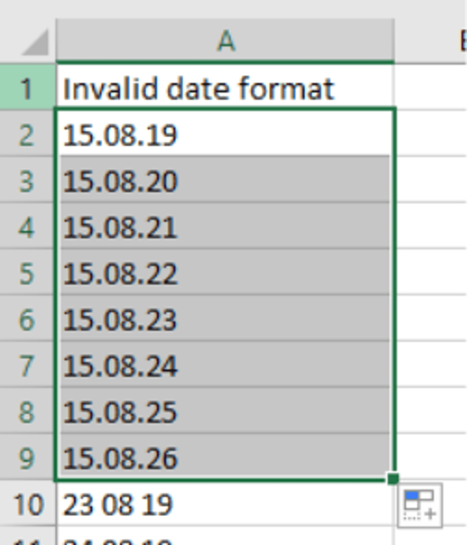
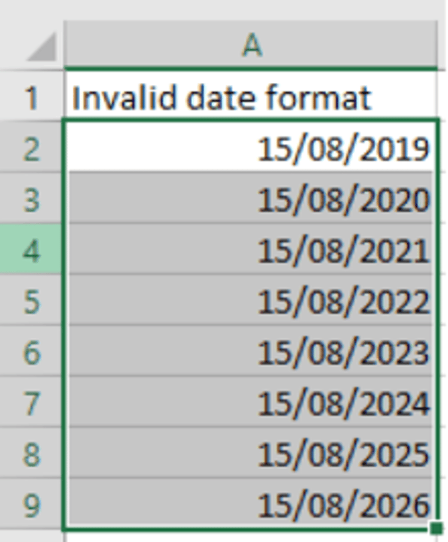
When trying to convert a date into a month/day/year format, you might be unable to because Excel will read the selected value as a string of text, not a valid numerical date.

But how do you know if your entry is being read as a “text date” instead of an accepted numerical Excel date?

• Text dates are left-aligned. Excel dates are right-aligned by default.
• The status bar shows count when multiple text format dates are selected. When multiple Excel dates are selected, the status bar should display average, count, and sum.
• Text dates might have a leading apostrophe in the formula bar.

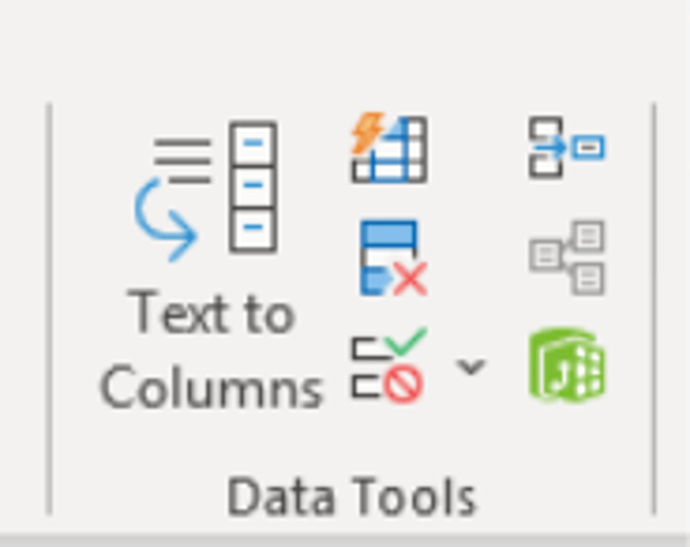
Using the Text to Columns Feature, you can correct text date formats by following the steps below:

1. Select the cells containing the dates.

   
2. Click the Data tab in the Excel Ribbon.

3. Choose the Text to Columns feature to open the Wizard.

   

4. Click Delimited, then select the delimiters applicable to your date format.

   

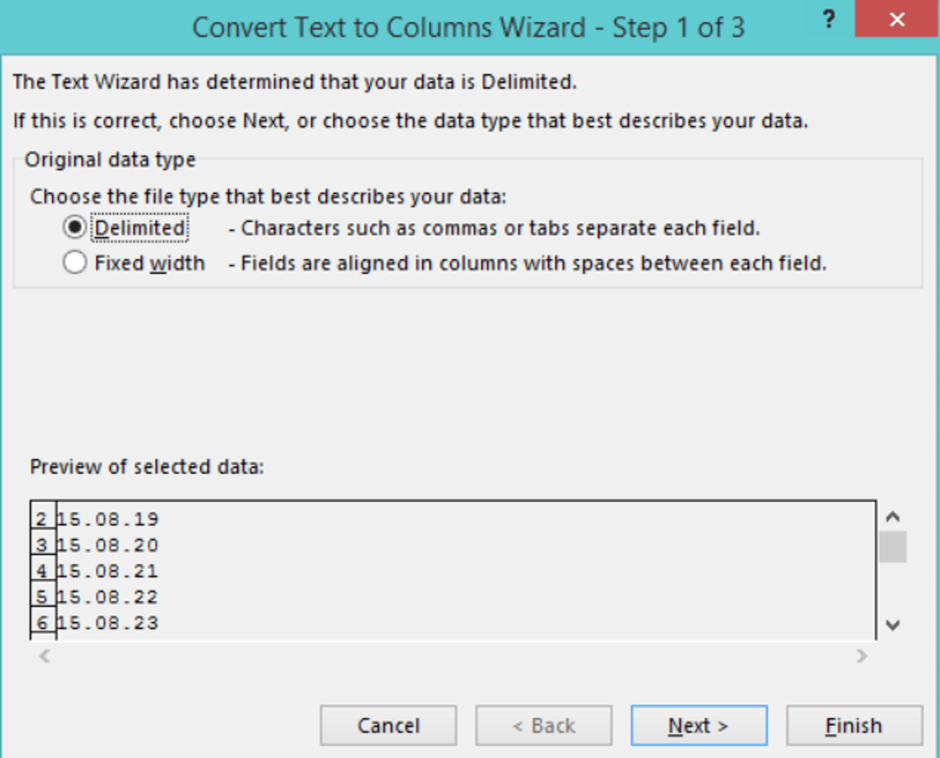
5. Under the Column Data Format option choose Date, then select the day/month/year format you desire from the list.

   

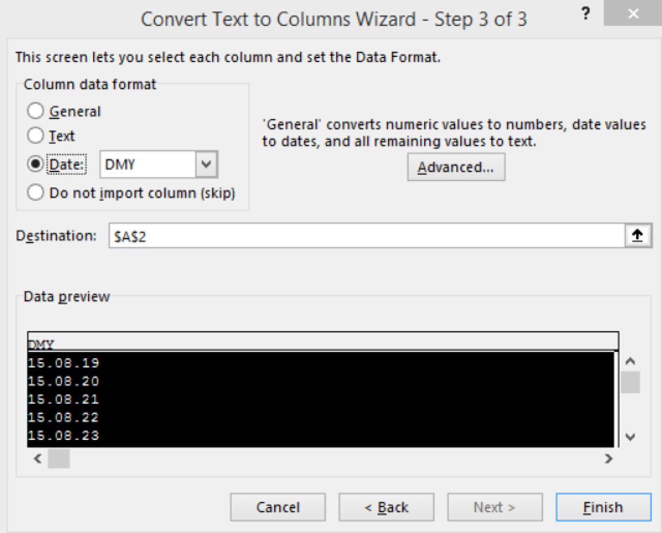
6. Click Finish, to convert the text dates to real dates.

   

Did you know: You can create powerful dashboards and data visualizations using your Excel spreadsheets in Klipfolio. Klipfolio lets you build custom dashboards using all of your data.

Excel Tip 4: How to Join Tables Using Power Query For High-Powered Data Analysis

Having all the data you need in a single worksheet is rare. Data is often scattered across multiple worksheets and workbooks, leaving the formidable task of collating and processing down to you.

Fortunately, Excel’s Power Query tool - known as Get & Transform in Excel 2016 and Excel 2019 - is amazing at combining and(you guessed it) transforming data from multiple sources into the format you need.

With Power Query, you can join 2 tables into 1 or combine data from multiple tables with corresponding data in columns. Here’s an in-depth Power Query 101 guide to get you started. Before you begin though, note the following facts about joining tables in Power Query:

• Tables should have a unique identifier, at least one common column.
• Data must be tidy and columns should contain unique values with no repeat data.
• You can use source tables from the same sheet or seperate worksheets.

Mini Excel Tip: You have to instruct excel to refresh joined tables. Power Query tables do not update automatically.

Excel Tip 5: How To Transform Messy Information Into “Squeaky-Clean” Data

When processing large amounts of information, bumping into dirty data is inevitable.

Trailing spaces, misspelled words, and improper cases and format look unprofessional and make information hard to read. They can even interfere with computing functions, preventing Excel from displaying your data correctly.

Cleaning up data isn’t nearly as hard as cleaning up in real life (hurray for that). Using the Excel tips and tricks below, you can turn messy information into sparkling data.

1. Formatting data: After importing data from an external source, you will usually have to clear the formatting before usage. To do so, simply select the data set, click on the clear dropdown, and then select clear formats.
2. Trailing spaces: The TRIM function is a quick alternative to the painful find-and-delete method for removing spaces. It removes leading, trailing and in-between spaces except for a single space between words. Syntax =TRIM(text)

3. Ambiguous/misspelled words: The Search/Replace function allows you to locate a specific word and replace it with a new one. Hit CTRL+F to summon the dialogue.

   Mini Excel Tip: You have to instruct excel to refresh joined tables. Power Query tables do not update automatically.

4. Inconsistent Case: Avoid manually correcting capitals and lower cases with the case formulas below:

   -Proper () – Converts all Text into Proper Case

   -Lower () – Converts all text into Lower Case

   -Upper () – Converts all text into Upper Case

Mini Excel Tip: By recording a macro or writing code, you can automate parts of the data cleaning process. If you don’t have the time or don’t want to learn macros, you can use external add-ins written by third-party vendors.

Fun Excel Tips & Tricks: The Most Useful Keyboard Shortcuts

Lastly, we’ve listed some fun Excel keyboard shortcuts to make you look like a true professional and impress your colleagues (hopefully they’ll offer to buy you a beer in exchange for your knowledge).

• “CTRL + 1”: Shortcut into the “Format Cells” window
• “CTRL + K”: Insert a hyperlink
• “CTRL + SHIFT + T” : Sums a column of data and puts the total in the next cell
• “CTRL + ?”: Climbs to the top cell, or “CTRL + ?” to drop to the last cell
• “CTRL + -” : Deletes the column your cursor rests on and “CTRL + SHIFT + =” will add a new column
• “CTRL” + `”: Reveals all the formulas in the spreadsheet

Want More Horsepower In Your Excel Spreadsheet Reporting?

Discover Klipfolio! With over 55,000 data leaders relying upon us everyday, Klipfolio pulls in data from all your favourite apps from spreadsheets to SQL to anything with an API.

Here are some great resources to show you how to get more horsepower from spreadsheet data:

• How to Build an Excel Dashboard: Webinar
• Klipfolio Solutions Overview: Excel Reporting Tool
• Klipfolio Integration with Excel
• Working with Excel and OneDrive: Video Tutorial

Happy reading and as usual, please feel free to reach out if you think I missed anything in this blog.